Graphical Features of Exponential Functions

Graphically, in the function f(x) = ab^x.

• a is the vertical intercept of the graph.
• b determines the rate at which the graph grows:
  • the function will increase if b > 1,
  • the function will decrease if 0 < b < 1.
• The graph will have a horizontal asymptote at y = 0. The graph will be concave up if a>0; concave down if a < 0.
• The domain of the function is all real numbers.
• The range of the function is (0,∞) if a > 0, and (−∞,0) if a < 0.

When sketching the graph of an exponential function, it can be helpful to remember that the graph will pass through the points (0, a) and (1, ab). The value b will determine the function's long run behavior:

• If b > 1, as x → ∞, f(x) → ∞, and as x → −∞, f(x) → 0.
• If 0 < b < 1, as x → ∞, f(x) → 0, and as x → –∞, f(x) → ∞.

Example 6

Sketch a graph of [latex-display]\displaystyle{f{{({x})}}}={4}{(\frac{{1}}{{3}})}^{{x}}[/latex-display] This graph will have a vertical intercept at (0,4), and pass through the point [latex]\displaystyle{({1},frac{{4}}{{3}})}[/latex]. Since b < 1, the graph will be decreasing towards zero. Since a > 0, the graph will be concave up.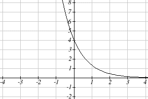 We can also see from the graph the long run behavior: as x → ∞ , f(x) → 0, and as x → –∞, f(x) → ∞. To get a better feeling for the effect of a and b on the graph, examine the sets of graphs below. The first set shows various graphs, where a remains the same and we only change the value for b. Notice that the closer the value of is to 1, the less steep the graph will be. 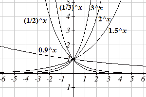Changing the value of b . In the next set of graphs, a is altered and our value for b remains the same. 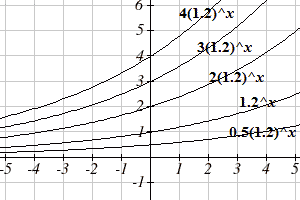Changing the value of a. Notice that changing the value for a changes the vertical intercept. Since a is multiplying the b^x term, a acts as a vertical stretch factor, not as a shift. Notice also that the long run behavior for all of these functions is the same because the growth factor did not change and none of these values introduced a vertical flip. Try it for yourself using this applet.

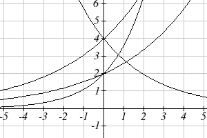
Example 7

Match each equation with its graph.

• [latex]\displaystyle{f{{({x})}}}={2}{({1.3})}^{{x}}[/latex]
• [latex]\displaystyle{g{{({x})}}}={2}{({1.8})}^{{x}}[/latex]
• [latex]\displaystyle{h}{({x})}={4}{({1.3})}^{{x}}[/latex]
• [latex]\displaystyle{k}{({x})}={4}{({0.7})}^{{x}}[/latex]

The graph of k(x) is the easiest to identify, since it is the only equation with a growth factor less than one, which will produce a decreasing graph. The graph of h(x) can be identified as the only growing exponential function with a vertical intercept at (0,4). The graphs of f(x) and g(x) both have a vertical intercept at (0,2), but since g(x) has a larger growth factor, we can identify it as the graph increasing faster.

---

Shana Calaway, Dale Hoffman, and David Lippman, Business Calculus, " 1.7: Exponential Functions," licensed under a CC-BY license.