Hamiltonian Circuits
Learning Outcomes
- Determine whether a graph has an Euler path and/ or circuit
- Use Fleury's algorithm to find an Euler circuit
- Add edges to a graph to create an Euler circuit if one doesn't exist
- Identify whether a graph has a Hamiltonian circuit or path
- Find the optimal Hamiltonian circuit for a graph using the brute force algorithm, the nearest neighbor algorithm, and the sorted edges algorithm
- Identify a connected graph that is a spanning tree
- Use Kruskal's algorithm to form a spanning tree, and a minimum cost spanning tree
Hamiltonian Circuits and the Traveling Salesman Problem
In the last section, we considered optimizing a walking route for a postal carrier. How is this different than the requirements of a package delivery driver? While the postal carrier needed to walk down every street (edge) to deliver the mail, the package delivery driver instead needs to visit every one of a set of delivery locations. Instead of looking for a circuit that covers every edge once, the package deliverer is interested in a circuit that visits every vertex once.Hamiltonian Circuits and Paths
Example
Example
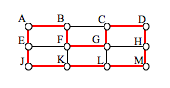
Does a Hamiltonian path or circuit exist on the graph below? We can see that once we travel to vertex E there is no way to leave without returning to C, so there is no possibility of a Hamiltonian circuit. If we start at vertex E we can find several Hamiltonian paths, such as ECDAB and ECABD
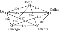 question can be framed like this: Suppose a salesman needs to give sales pitches in four cities. He looks up the airfares between each city, and puts the costs in a graph. In what order should he travel to visit each city once then return home with the lowest cost?
To answer this question of how to find the lowest cost Hamiltonian circuit, we will consider some possible approaches. The first option that might come to mind is to just try all different possible circuits.
question can be framed like this: Suppose a salesman needs to give sales pitches in four cities. He looks up the airfares between each city, and puts the costs in a graph. In what order should he travel to visit each city once then return home with the lowest cost?
To answer this question of how to find the lowest cost Hamiltonian circuit, we will consider some possible approaches. The first option that might come to mind is to just try all different possible circuits.
Brute Force Algorithm (a.k.a. exhaustive search)
Example
Apply the Brute force algorithm to find the minimum cost Hamiltonian circuit on the graph below.
| Circuit | Weight |
| ABCDA | 4+13+8+1 = 26 |
| ABDCA | 4+9+8+2 = 23 |
| ACBDA | 2+13+9+1 = 25 |

Number of Possible Circuits
Example
| Cities | Unique Hamiltonian Circuits |
| 9 | 8!/2 = 20,160 |
| 10 | 9!/2 = 181,440 |
| 11 | 10!/2 = 1,814,400 |
| 15 | 14!/2 = 43,589,145,600 |
| 20 | 19!/2 = 60,822,550,204,416,000 |
Nearest Neighbor Algorithm (NNA)
Example
The resulting circuit is ADCBA with a total weight of [latex]1+8+13+4 = 26[/latex].
Example
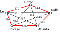 LA to Chicago: $100
Chicago to Atlanta: $75
Atlanta to Dallas: $85
Dallas to Seattle: $120
Total cost: $450
In this case, nearest neighbor did find the optimal circuit.
LA to Chicago: $100
Chicago to Atlanta: $75
Atlanta to Dallas: $85
Dallas to Seattle: $120
Total cost: $450
In this case, nearest neighbor did find the optimal circuit.
Example
Starting at vertex A resulted in a circuit with weight 26.
Starting at vertex B, the nearest neighbor circuit is BADCB with a weight of 4+1+8+13 = 26. This is the same circuit we found starting at vertex A. No better.
Starting at vertex C, the nearest neighbor circuit is CADBC with a weight of 2+1+9+13 = 25. Better!
Starting at vertex D, the nearest neighbor circuit is DACBA. Notice that this is actually the same circuit we found starting at C, just written with a different starting vertex.
The RNNA was able to produce a slightly better circuit with a weight of 25, but still not the optimal circuit in this case. Notice that even though we found the circuit by starting at vertex C, we could still write the circuit starting at A: ADBCA or ACBDA.
Try It
The table below shows the time, in milliseconds, it takes to send a packet of data between computers on a network. If data needed to be sent in sequence to each computer, then notification needed to come back to the original computer, we would be solving the TSP. The computers are labeled A-F for convenience.| A | B | C | D | E | F | |
| A | -- | 44 | 34 | 12 | 40 | 41 |
| B | 44 | -- | 31 | 43 | 24 | 50 |
| C | 34 | 31 | -- | 20 | 39 | 27 |
| D | 12 | 43 | 20 | -- | 11 | 17 |
| E | 40 | 24 | 39 | 11 | -- | 42 |
| F | 41 | 50 | 27 | 17 | 42 | -- |
Example
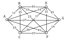
The cheapest edge is AD, with a cost of 1. We highlight that edge to mark it selected.

 For the third edge, we’d like to add AB, but that would give vertex A degree 3, which is not allowed in a Hamiltonian circuit. The next shortest edge is CD, but that edge would create a circuit ACDA that does not include vertex B, so we reject that edge. The next shortest edge is BD, so we add that edge to the graph.
 BAD
BAD BAD
BAD OK
OK While the Sorted Edge algorithm overcomes some of the shortcomings of NNA, it is still only a heuristic algorithm, and does not guarantee the optimal circuit.
Example
| Ashland | Astoria | Bend | Corvallis | Crater Lake | Eugene | Newport | Portland | Salem | Seaside | |
| Ashland | - | 374 | 200 | 223 | 108 | 178 | 252 | 285 | 240 | 356 |
| Astoria | 374 | - | 255 | 166 | 433 | 199 | 135 | 95 | 136 | 17 |
| Bend | 200 | 255 | - | 128 | 277 | 128 | 180 | 160 | 131 | 247 |
| Corvallis | 223 | 166 | 128 | - | 430 | 47 | 52 | 84 | 40 | 155 |
| Crater Lake | 108 | 433 | 277 | 430 | - | 453 | 478 | 344 | 389 | 423 |
| Eugene | 178 | 199 | 128 | 47 | 453 | - | 91 | 110 | 64 | 181 |
| Newport | 252 | 135 | 180 | 52 | 478 | 91 | - | 114 | 83 | 117 |
| Portland | 285 | 95 | 160 | 84 | 344 | 110 | 114 | - | 47 | 78 |
| Salem | 240 | 136 | 131 | 40 | 389 | 64 | 83 | 47 | - | 118 |
| Seaside | 356 | 17 | 247 | 155 | 423 | 181 | 117 | 78 | 118 | - |
To see the entire table, scroll to the right
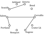
Using NNA with a large number of cities, you might find it helpful to mark off the cities as they’re visited to keep from accidently visiting them again. Looking in the row for Portland, the smallest distance is 47, to Salem. Following that idea, our circuit will be:
Using Sorted Edges, you might find it helpful to draw an empty graph, perhaps by drawing vertices in a circular pattern. Adding edges to the graph as you select them will help you visualize any circuits or vertices with degree 3.
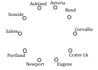
We start adding the shortest edges:
Seaside to Astoria 17 miles
Corvallis to Salem 40 miles
Portland to Salem 47 miles
Corvallis to Eugene 47 miles
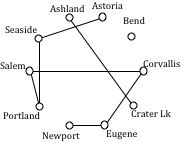
Newport to Astoria (reject – closes circuit)
Newport to Bend 180 miles
Bend to Ashland 200 miles
At this point the only way to complete the circuit is to add:
Crater Lk to Astoria 433 miles. The final circuit, written to start at Portland, is:
Portland, Salem, Corvallis, Eugene, Newport, Bend, Ashland, Crater Lake, Astoria, Seaside, Portland. Total trip length: 1241 miles.
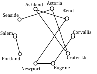
While better than the NNA route, neither algorithm produced the optimal route. The following route can make the tour in 1069 miles:
Portland, Astoria, Seaside, Newport, Corvallis, Eugene, Ashland, Crater Lake, Bend, Salem, Portland
Try It
Licenses & Attributions
CC licensed content, Original
- Revision and Adaptation. Provided by: Lumen Learning License: CC BY: Attribution.
CC licensed content, Shared previously
- Hamiltonian circuits . Authored by: LIPPMAN, DAVID. License: CC BY: Attribution.
- TSP by brute force . Authored by: OCLPhase2. License: CC BY: Attribution.
- Number of circuits in a complete graph . Authored by: OCLPhase2. License: CC BY: Attribution.
- Nearest Neighbor ex2 . Authored by: OCLPhase2. License: CC BY: Attribution.
- Sorted Edges ex 2 . Authored by: OCLPhase2. License: CC BY: Attribution.
- Kruskal's ex 1 . Authored by: OCLPhase2. License: CC BY: Attribution.
- Kruskal's from a table . Authored by: OCLPhase2. License: CC BY: Attribution.
