Graph Radical Functions
Learning Outcome
- Graph radical functions using tables and transformations
| x | f(x) |
|---|---|
| [latex]0[/latex] | [latex]0[/latex] |
| [latex]1[/latex] | [latex]1[/latex] |
| [latex]4[/latex] | [latex]2[/latex] |
| [latex]9[/latex] | [latex]3[/latex] |
| [latex]16[/latex] | [latex]4[/latex] |

Example
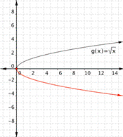
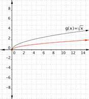
Match each of the following functions to the graph that it represents. a) [latex]f(x)=-\sqrt{x}[/latex] b)[latex]f(x)=2\sqrt{x}[/latex] c) [latex]f(x)=\dfrac{1}{2}\sqrt{x}[/latex] 1)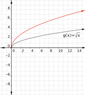 2)
2)
 3)
3)
Answer:
Function a) goes with graph 2)
Function b) goes with graph 1)
Function c) goes with graph 3)
Function a) [latex]f(x)=-\sqrt{x}[/latex] means that all the outputs will be negative - the function is the negative of the square roots of the input. This will give the other half of the parabola on its side. Therefore graph 2) goes with the function [latex]f(x)=-\sqrt{x}[/latex].
 Function b) [latex]f(x)=2\sqrt{x}[/latex] means take the square root of all the inputs, then multiply by two, so the outputs will be larger than the outputs for [latex]\sqrt{x}[/latex]. Graph 1) goes with the function [latex]f(x)=2\sqrt{x}[/latex].
 Function c) [latex]f(x)=\dfrac{1}{2}\sqrt{x}[/latex] means take the squat=re root of the inputs then multiply by [latex]\Large\frac{1}{2}[/latex]. The outputs will be smaller than the outputs for [latex]\sqrt{x}[/latex]. Graph 3) goes with the function [latex]f(x)=\dfrac{1}{2}\sqrt{x}[/latex].

Example
Match each of the following functions to the graph that it represents. a) [latex] f(x)=\sqrt{x}+3[/latex] b)[latex] f(x)=\sqrt{x}-2[/latex] 1)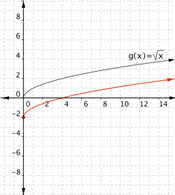 2)
2)
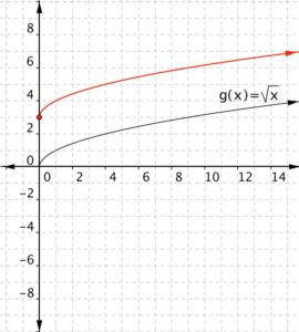
Answer:
Function a) goes with graph 2)
Function b) goes with graph 1)
Function a) [latex] f(x)=\sqrt{x}+3[/latex] means take the square root of all the inputs and add three, so the out puts will be greater than those for [latex]\sqrt{x}[/latex], therefore graph 2) goes with this function.
 Function b) [latex]f(x)=\sqrt{x}-2[/latex] means take the square root of the input then subtract two. The outputs will be less than those for [latex]\sqrt{x}[/latex], therefore graph 1) goes with this function.

Example
Match each of the following functions to the graph that it represents. a) [latex]f(x)=\sqrt{x+1}[/latex] b)[latex]f(x)=\sqrt{x-2}[/latex] 1)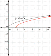 2)
2)
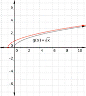
Answer:
Function a) matches graph 2)
Function b) matches graph 1)
Function a) [latex]f(x)=\sqrt{x+1}[/latex] adds one to the inputs before the square root is taken. The outputs will be greater, so it ends up looking like a shift to the left. Graph 2) matches this function.
 Function b) [latex]f(x)=\sqrt{x-2}[/latex] means subtract before the square root is taken. This makes the outputs less than they would be for the standard [latex]\sqrt{x}[/latex], and looks like a shift to the right. Graph 1) matches this function.

Example
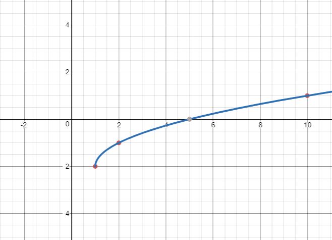
Graph [latex] f(x)=-2+\sqrt{x-1}[/latex].Answer: Before making a table of values, look at the function equation to get a general idea about what the graph should look like. Inside the square root, you are subtracting [latex]1[/latex], so the graph will move to the right [latex]1[/latex] from the basic [latex] f(x)=\sqrt{x}[/latex] graph. You are also adding [latex]−2[/latex] outside the square root, so the graph will move down two from the basic [latex] f(x)=\sqrt{x}[/latex] graph. Create a table of values. Choose values that will make your calculations easy. You want [latex]x–1[/latex] to be a perfect square ([latex]0, 1, 4, 9[/latex], and so on) so you can take the square root.
| x | f(x) |
|---|---|
| [latex]1[/latex] | [latex]−2[/latex] |
| [latex]2[/latex] | [latex]−1[/latex] |
| [latex]5[/latex] | [latex]0[/latex] |
| [latex]10[/latex] | [latex]1[/latex] |
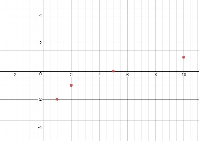 Connect the points as best you can using a smooth curve.
Licenses & Attributions
CC licensed content, Original
- Revision and Adaptation. Provided by: Lumen Learning License: CC BY: Attribution.
CC licensed content, Shared previously
- Chapter 17. Authored by: Monterey Institute for Technology and Education. Located at: https://www.nroc.org/. License: CC BY: Attribution.
